
In questo secondo tutorial di Code_Aster verrà trattato il tema delle deformazioni indotte da uno shock termico o da un generico raffreddamento brusco in un componente metallico, sarà pertanto necessario accoppiare l'analisi termica ad un'analisi meccanica (sforzo-deformazione).
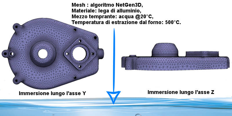
Durante la tempra (raffreddamento improvviso) di componenti dalla geometria complessa è importante trovare la disposizione o orientamento che minimizza le deformazioni e le tensioni residue. Nella realtà il raffreddamento non è omogeneo; è impossibile infatti che tutte le facce del componente vengono raffreddate nello stesso identico istante. Per questo motivo è opportuno inserire nella simulazione, come condizione al contorno, la direzione e la velocità di immersione nel bagno di tempra.
Nel tutorial viene introdotta una funzione arbitraria per la gestione della condizione al contorno superficiale durante l'immersione. La funzione generata è una funzione logistica in quanto l'obiettivo dichiarato è avere una variazione brusca del coefficiente_h ma non istantanea. Tale funzione ha come variabili la direzione di immersione (coordinata Z ad esempio) e il tempo (INST). Il componente utilizzato, un generico carter di forma mediamente complessa, è stato scaricato da GrabCad .
Sono state simulate due direzioni di immersione, scelte in modo arbitrario, allo scopo di evidenziare il raffreddamento non omogeneo e conseguentemente la differente distribuzione di tensioni residue nel pezzo alla fine del trattamento.
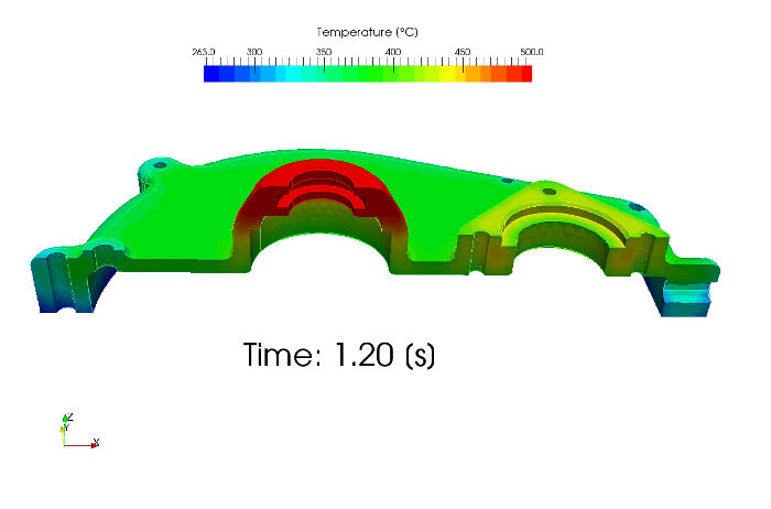
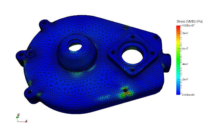
RISULTATI
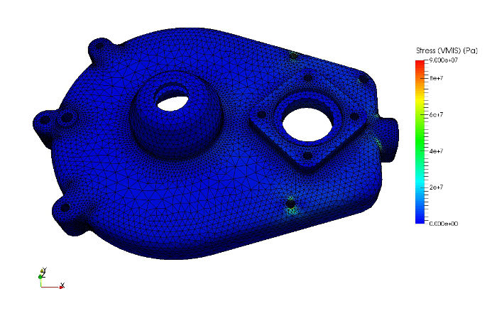
CONCLUSIONI
Come era possibile aspettarsi, la direzione lungo Y genera maggiori tensioni residue all'interno del pezzo rispetto alla direzione Z. La disposizione "di piatto" (lungo Z) del carter in lega d'alluminio durante il ciclo di trattamento sembra pertanto da preferirsi per diminuire sia le deformazioni sia gli stress residui da tempra
Molte delle informazioni teoriche riguardo le funzioni utilizzate nel file di comando per queste simulazioni sono eccellentemente descritte nel tutorial di Paul Carrico
FILE DI COMANDO DELLA SIMULAZIONE IN CODE_ASTER / COMMAND FILE
DEBUT();
#MESH IMPORT: lire_maillage per importare la mesh in formato MED
mesh=LIRE_MAILLAGE(FORMAT='MED',);
#MESH REFINING / RAFFINAMENTO DELLA MESH
#
#MACR_ADAP_MAIL = mesh refining homogeneous (RAFFINEMENT_UNIFORME), the aim is to provide a refined linear mesh for thermal calculations.
MACR_ADAP_MAIL(MAILLAGE_N=mesh,
MAILLAGE_NP1=CO('mesh_2'),
ADAPTATION='RAFFINEMENT_UNIFORME',);
#-------------------------------
#DIPPING FORMULA / FORMULA PER LA SIMULAZIONE DELL'IMMERSIONE
#
#Using a logistic function function of space and time to simulate the water h-coefficient affecting linearly the componenet along the dipping direction (i.e. X axys)
#dipping time = t_im = [s]
#dimensions d_min and d_max = bounding box values of the model along the desired dipping direction = [m]
#v_dip = dipping velocity [m/s]
#h_max = water coef. h value [W / m^2 K]
#-------------------------------
h_max = 3000;
d_min = 0;
d_max = 0.047;
v_dip = 0.03;
t_im = 1;
coef_h = FORMULE(VALE='(h_max)/(1+ exp(-30*(INST-(Z-d_min)/(v_dip))))',
NOM_PARA=('Z','INST',),);
t_ext=DEFI_FONCTION(
NOM_PARA='INST',
VALE=(0.0 , 20.0 ,),
PROL_DROITE='CONSTANT',
PROL_GAUCHE='CONSTANT',);
#-------------------------------
#MATERIAL DEFINITION / DEFINIZIONE MATERIALE
#funzione DEFI_MATERIAU.
#THER = thermal properties / proprieta' termiche !!! WARNING !!!! RHO_CP = density * specific heat [J/(m^3 *K)]
#ELAS = elastic properties, Elastic modulus, NU poisson's modulus, ALPHA = thermal linear deformation [1/K]
#ECRO_LINE = plastic properties
#-------------------------------
mate=DEFI_MATERIAU(ELAS=_F(E=76000000000.0,
NU=0.3,
RHO=2700.0,
ALPHA=2.25e-05,),
ECRO_LINE=_F(D_SIGM_EPSI=7e+08,
SY=100e+06,),
THER=_F(LAMBDA=120.0,
RHO_CP=2430000.0,),);
#-------------------------------
# MATERIAL DOMAIN / DEFINIZIONE DEL DOMINIO DEL MATERIALE ---------
#command AFFE_MATERIAU . Define which part (TOUT=OUI) of the mesh (MAILLAGE) is affected by material properties (MATER)
#-------------------------------
affe_t=AFFE_MATERIAU(MAILLAGE=mesh_2,
AFFE=_F(TOUT='OUI',
MATER=mate,),
AFFE_VARC=_F(TOUT='OUI',
NOM_VARC='TEMP',
VALE_REF=20.0,),);
#-------------------------------
#MODEL DEFINITION / DEFINIZIONE DEL MODELLO
#command AFFE_MODELE , definition of the phisical domain (PHENOMENE=thermique)
#-------------------------------
m_ter=AFFE_MODELE(MAILLAGE=mesh_2,
AFFE=_F(TOUT='OUI',
PHENOMENE='THERMIQUE',
MODELISATION='3D_DIAG',),);
#-------------------------------
#THERMAL BOUNDARY CONDITION / CONDIZIONI AL CONTORNO TERMICHE
#Boundary Exchange / Scambio Termico alla superficie (ECHANGE)
#In this water quenching case a static mean exchange coefficient (COEF_H) [W/(m^2 * K)] is used with a defined water temperature (TEMP_EXT)
#-------------------------------
char_t=AFFE_CHAR_THER_F(MODELE=m_ter,
ECHANGE=_F(GROUP_MA='quench',
COEF_H=coef_h,
TEMP_EXT=t_ext,),);
#-------------------------------
#TIME TRANSIENT DEFINITION / DEFINIZIONE DELLA LISTA DEGLI ISTANTI DI CALCOLO
#Starting from a list of number defined with DEFI_LIST_REEL in several intervals, the intervals have smaller timesteps during the firsts seconds of the simulation
#-------------------------------
tempo=DEFI_LIST_REEL(DEBUT=0.0,
INTERVALLE=(_F(JUSQU_A=2.0,
PAS=0.1,),
_F(JUSQU_A=10.0,
PAS=0.25,),),);
inst=DEFI_LIST_INST(DEFI_LIST=_F(METHODE='AUTO',
LIST_INST=tempo,
PAS_MINI=0.005,
PAS_MAXI=3.0,),
ADAPTATION=_F(EVENEMENT='TOUT_INST',
MODE_CALCUL_TPLUS='IMPLEX',),);
#-------------------------------
#THERMAL SOLVER / RISOLUZIONE DEL PROBLEMA TERMICO
#since this is a linear case the command for the resolution is THER_LINEARE, the initial state (ETAT_INIT) is defined in temperature (500 C) at the time 0.0 (INST_ETAT_INIT)
#-------------------------------
t_lin=THER_LINEAIRE(MODELE=m_ter,
CHAM_MATER=affe_t,
EXCIT=_F(CHARGE=char_t,),
ETAT_INIT=_F(VALE=500.0,
INST_ETAT_INIT=0.0,),
INCREMENT=_F(LIST_INST=inst,
INST_INIT=0.0,),
SOLVEUR=_F(METHODE='MULT_FRONT',),
PARM_THETA=0.57,);
#----------------- END OF THERMAL STUDY --------------------------
#
#----------------- START OF MECHANICAL STUDY ------------------
#
#-------------------------------
#MESH CONVERSION FROM LINEAR (best for thermal) TO QUADRATIC (best for mechanical)
#CREA_MAILLAGE mesh --> mesh_q
# LINE_QUAD --> TOUT = OUI
#-------------------------------
mesh_q=CREA_MAILLAGE(MAILLAGE=mesh,
LINE_QUAD=_F(TOUT='OUI',),);
#-------------------------------
#MODEL DEFINITION / DEFINIZIONE DEL MODELLO
#command AFFE_MODELE , definition of the phisical domain (PHENOMENE=mecanique) using the quadratic mesh mesh_q
#MODELIZATION = 3D ( better than 3D_DIAG for stress-strains)
#-------------------------------
m_meca=AFFE_MODELE(MAILLAGE=mesh_q,
AFFE=_F(TOUT='OUI',
PHENOMENE='MECANIQUE',
MODELISATION='3D',),);
#-------------------------------
#USE THE THERMAL RESULTS AS INPUTS FOR MECHANICAL CALCULATIONS
#
#PROJ_CHAMP : from thermal model to mechanical model (MODELE_1 , MODELE_2) using VIS_A_VIS TOUT1 and TOUT2 = OUI , all the elements
#-------------------------------
proj=PROJ_CHAMP(PROJECTION='OUI',
RESULTAT=t_lin,
MODELE_1=m_ter,
MODELE_2=m_meca,
VIS_A_VIS=_F(TOUT_1='OUI',
TOUT_2='OUI',
CAS_FIGURE='3D',),);
#-------------------------------
#MATERIAL DOMAIN / DEFINIZIONE DEL DOMINIO DEL MATERIALE
#command AFFE_MATERIAU . Define which part (TOUT=OUI) of the mesh (MAILLAGE) is affected by material properties (MATER) and by the calculated therm history ( AFFE_VARC --> EVOL ) projected before into the new mesh.
#
#------IMPORTANT FOR NON-LINEAR behaviours ----
#AFFE_VARC is used to set the variable fo non linearity (TEMP) and the reference value (VALE_REF)
#-------------------------------
mat_m=AFFE_MATERIAU(MODELE=m_meca,
AFFE=_F(TOUT='OUI',
MATER=mate,),
AFFE_VARC=_F(NOM_VARC='TEMP',
EVOL=proj,
VALE_REF=500.0,),);
#-------------------------------
#MECHANICAL BOUNDARY CONDITIONS
#
#FIXED NODE : the reference node (GROUP_NO) of the component in order to simulate a free-deformable object (something just placed on a surface and not fixed to anything)
#
#NB In case of SYMMETRY : the section/face (GROUP_MA) across the symmetry plan should be fixed regarding movements perpendicularly to the simmetry-plane, i.e. simmetryplane : XZ-plane --> section: DY = 0
#-------------------------------
char_m=AFFE_CHAR_MECA(MODELE=m_meca,
DDL_IMPO=(_F(GROUP_NO='dxdydz',
DX=0.0,
DY=0.0,
DZ=0.0,),
_F(GROUP_NO='dydz',
DY=0.0,
DZ=0.0,),
_F(GROUP_NO='dxdy',
DX=0.0,
DY=0.0,),),);
#-------------------------------
#MECHANICAL SOLVER / RISOLUZIONE DEL DOMINIO MECCANICO
#
#STAT_NON_LINE since it's a non-linear problem; it's very important to choos the right COMPORTEMENT according to the material behaviour choosen before (ECRO_LINE --> VMIS_ISOT_LINE ) and the right strain algorithm (PETIT_REAC) in this case.
#
#CONVERGENCE TIP = to increase convergence it's possible to recalculate the Newton matrix at every iteration: NEWTON --> REAC_ITER = 1
#
#-------------------------------
meca=STAT_NON_LINE(MODELE=m_meca,
CHAM_MATER=mat_m,
EXCIT=_F(CHARGE=char_m,),
COMPORTEMENT=_F(TOUT='OUI',
RELATION='VMIS_ISOT_LINE',
DEFORMATION='PETIT_REAC',),
INCREMENT=_F(LIST_INST=tempo,
INST_INIT=0.0,),
METHODE='NEWTON',
NEWTON=_F(PREDICTION='ELASTIQUE',
MATRICE='TANGENTE',
REAC_ITER=1,),
CONVERGENCE=_F(ITER_GLOB_MAXI=20,),
SOLVEUR=_F(METHODE='MULT_FRONT',),);
#-------------------------------
#STRESS STRAIN CALCULATION / ESTRAPOLAZIONE DELLE TENSIONI E DELLE DEFORMAZIONI
#
#Using CALC_CHAMP is possible to save at the node (XXX_NOEU, useful since can directly be displayed in Paraview) several fields calculated from the mechanical resolution (STAT_NON_LINE).
#SIGM = STRESSES
#EPSI = TOTAL STRAIN
#EPME = ONLY MECHANICAL STRAIN (no thermal inducted strain)
#SIEQ = EQUIVALENT STRESS (TRESCA,VonMISes,...)
#VARI = specific internal variable of the solution (V1 = PLASTICIZATION)
#
#-------------------------------
epsi=CALC_CHAMP(MODELE=m_meca,
CHAM_MATER=mat_m,
RESULTAT=meca,
TOUT_ORDRE='OUI',
EXCIT=_F(CHARGE=char_m,),
CONTRAINTE='SIGM_NOEU',
DEFORMATION=('EPSI_NOEU','EPME_NOEU',),
CRITERES='SIEQ_NOEU',
VARI_INTERNE='VARI_NOEU',);
#-------------------------------
#SAVING RESULTS / SALVATAGGIO DEI RISULTATI
#The data calculated in THER_LINEAIRE, defined by the command RESU, are saved in MED format.
#-------------------------------
IMPR_RESU(FORMAT='MED',
RESU=(_F(MAILLAGE=mesh_2,
RESULTAT=t_lin,),
_F(MAILLAGE=mesh_q,
RESULTAT=meca,),
_F(MAILLAGE=mesh_q,
RESULTAT=epsi,),),);
FIN();